
Package Summary
| Tags | No category tags. |
| Version | 0.4.0 |
| License | BSD |
| Build type | AMENT_CMAKE |
| Use | RECOMMENDED |
Repository Summary
| Description | |
| Checkout URI | https://github.com/autowarefoundation/autoware_tools.git |
| VCS Type | git |
| VCS Version | main |
| Last Updated | 2025-12-17 |
| Dev Status | UNKNOWN |
| Released | UNRELEASED |
| Tags | No category tags. |
| Contributing |
Help Wanted (-)
Good First Issues (-) Pull Requests to Review (-) |
Package Description
Additional Links
Maintainers
- Cristian Gariboldi
Authors
Learning Based Vehicle Calibration
Getting Started
1. Installation
Navigate to autoware/src/tools/vehicle/learning_based_vehicle_calibration and install the required libraries:
# It is recommended to do this in a miniconda environment
# There are 2 stages: data collection and calibration.
# These requirements are only needed for the calibration step.
pip install -r requirements.txt
2. Longitudinal Dynamics
To start collecting data, launch in your workspace:
ros2 launch learning_based_vehicle_calibration calibration_launch.py
Inside this launch file there is a variable called ‘Recovery_Mode’, set to False by default. If while you were collecting data the software stopped for some reasons or something happened causing the interruption of your collection process, you can collect data recovering from previous breaking points by setting the variable to True. This way it will update the csv tables you have already started to collect without the need to start from scratch.
You can visualize the collection process from the terminal.
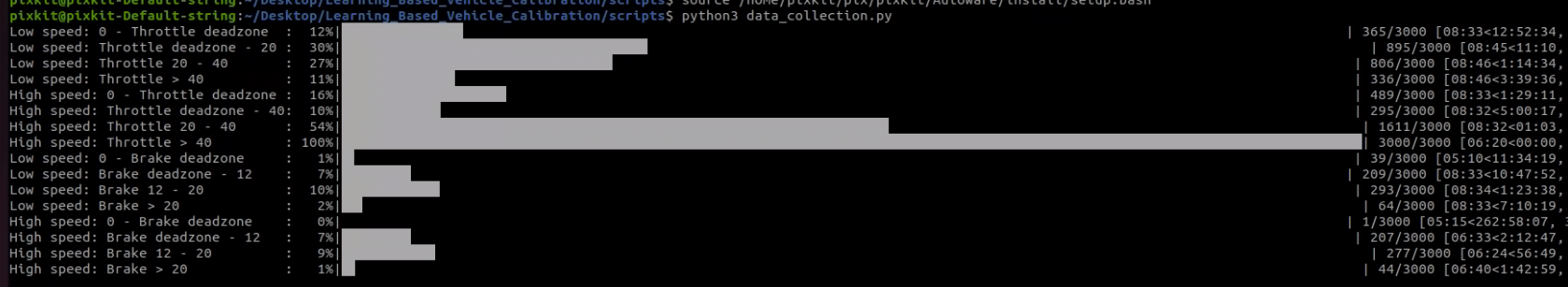
Otherwise, we built some custom messages for representing the progress that are being published on the following topics:
/scenarios_collection_longitudinal_throttling

/scenarios_collection_longitudinal_braking
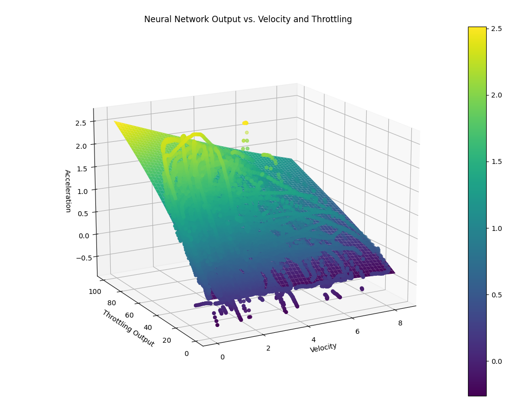
Once you have collected the data, in order to train and build your black box models, for both throttling and braking scenarios, launch:
ros2 launch learning_based_vehicle_calibration neural_network_launch.py
You will obtain the acceleration and braking calibration maps and visualize how the neural network fits the data:
Overview
Here we present the software structure, data collection, data preprocessing and neural network training and visualization about the end-to-end calibration of a vehicle, in two different scenarios:
- Normal driving conditions (longitudinal dynamics);
- Parking conditions (steering dynamics).
Input Data Software
Configure the Autoware to publish the necessary topics. Then launch Autoware.
It is recommended to record the topics we need to collect in order to train our model. The data we need to record are the pitch angle, the linear acceleration, the velocity, the braking and throttling values and the steering angle (make sure to modify the name of the topics according to your vehicle):
ros2 bag record /sensing/gnss/chc/pitch /vehicle/status/actuation_status /vehicle/status/steering_status /vehicle/status/velocity_status /vehicle/status/imu
- data_field: rosbag should contains brake_paddle, throttle_paddle, velocity, steering, imu and pitch
Data’s values and units of measure are as follows:
# brake paddle value (frome 0 to 1, float)
/vehicle/status/actuation_status -> status.brake_status
# throttle paddle value (frome 0 to 1, float)
/vehicle/status/actuation_status -> status.accel_status
# velocity value (unit is m/s, float)
/vehicle/status/velocity_status -> longitudinal_velocity
# steering value (from 0 to 0.5 [radians], float)
/vehicle/status/steering_status -> steering_tire_angle
# imu data(unit is rad/s or m/s)
/vehicle/status/imu -> linear_acceleration.x
# pitch angle (unit is degrees)
/sensing/gnss/chc/pitch -> data
When you run the calibration, data_monitor script is launched automatically.
Thanks to data_monitor script, we can make sure that we are receiving all the topics correctly, without any delay and any problem.
You can have a look at the following examples:
- if all the topics are published correctly, the scripts is going to print to terminal the following text, with the frequency of one second

- if instead one or more topics are not published or received correctly, or they are delayed, the script is going to warn you by printing to terminal for example the following text

1. Longitudinal Dynamics
Record Data Software Case
File truncated at 100 lines see the full file
Changelog for package learning_based_vehicle_calibration
0.4.0 (2025-11-16)
0.3.0 (2025-08-11)
- feat: add Learning-Based Accel/Brake Map Calibrator (#231)
- Contributors: CristianGariboldi
Package Dependencies
| Deps | Name |
|---|---|
| ament_cmake_auto | |
| rosidl_default_generators | |
| autoware_vehicle_msgs | |
| can_msgs | |
| rclpy | |
| ros2launch | |
| rosidl_default_runtime | |
| sensor_msgs | |
| std_msgs | |
| tier4_vehicle_msgs |
System Dependencies
Dependant Packages
Launch files
Services
Plugins
Recent questions tagged learning_based_vehicle_calibration at Robotics Stack Exchange
Package Summary
| Tags | No category tags. |
| Version | 0.4.0 |
| License | BSD |
| Build type | AMENT_CMAKE |
| Use | RECOMMENDED |
Repository Summary
| Description | |
| Checkout URI | https://github.com/autowarefoundation/autoware_tools.git |
| VCS Type | git |
| VCS Version | main |
| Last Updated | 2025-12-17 |
| Dev Status | UNKNOWN |
| Released | UNRELEASED |
| Tags | No category tags. |
| Contributing |
Help Wanted (-)
Good First Issues (-) Pull Requests to Review (-) |
Package Description
Additional Links
Maintainers
- Cristian Gariboldi
Authors
Learning Based Vehicle Calibration
Getting Started
1. Installation
Navigate to autoware/src/tools/vehicle/learning_based_vehicle_calibration and install the required libraries:
# It is recommended to do this in a miniconda environment
# There are 2 stages: data collection and calibration.
# These requirements are only needed for the calibration step.
pip install -r requirements.txt
2. Longitudinal Dynamics
To start collecting data, launch in your workspace:
ros2 launch learning_based_vehicle_calibration calibration_launch.py
Inside this launch file there is a variable called ‘Recovery_Mode’, set to False by default. If while you were collecting data the software stopped for some reasons or something happened causing the interruption of your collection process, you can collect data recovering from previous breaking points by setting the variable to True. This way it will update the csv tables you have already started to collect without the need to start from scratch.
You can visualize the collection process from the terminal.
Otherwise, we built some custom messages for representing the progress that are being published on the following topics:
/scenarios_collection_longitudinal_throttling

/scenarios_collection_longitudinal_braking
Once you have collected the data, in order to train and build your black box models, for both throttling and braking scenarios, launch:
ros2 launch learning_based_vehicle_calibration neural_network_launch.py
You will obtain the acceleration and braking calibration maps and visualize how the neural network fits the data:
Overview
Here we present the software structure, data collection, data preprocessing and neural network training and visualization about the end-to-end calibration of a vehicle, in two different scenarios:
- Normal driving conditions (longitudinal dynamics);
- Parking conditions (steering dynamics).
Input Data Software
Configure the Autoware to publish the necessary topics. Then launch Autoware.
It is recommended to record the topics we need to collect in order to train our model. The data we need to record are the pitch angle, the linear acceleration, the velocity, the braking and throttling values and the steering angle (make sure to modify the name of the topics according to your vehicle):
ros2 bag record /sensing/gnss/chc/pitch /vehicle/status/actuation_status /vehicle/status/steering_status /vehicle/status/velocity_status /vehicle/status/imu
- data_field: rosbag should contains brake_paddle, throttle_paddle, velocity, steering, imu and pitch
Data’s values and units of measure are as follows:
# brake paddle value (frome 0 to 1, float)
/vehicle/status/actuation_status -> status.brake_status
# throttle paddle value (frome 0 to 1, float)
/vehicle/status/actuation_status -> status.accel_status
# velocity value (unit is m/s, float)
/vehicle/status/velocity_status -> longitudinal_velocity
# steering value (from 0 to 0.5 [radians], float)
/vehicle/status/steering_status -> steering_tire_angle
# imu data(unit is rad/s or m/s)
/vehicle/status/imu -> linear_acceleration.x
# pitch angle (unit is degrees)
/sensing/gnss/chc/pitch -> data
When you run the calibration, data_monitor script is launched automatically.
Thanks to data_monitor script, we can make sure that we are receiving all the topics correctly, without any delay and any problem.
You can have a look at the following examples:
- if all the topics are published correctly, the scripts is going to print to terminal the following text, with the frequency of one second
- if instead one or more topics are not published or received correctly, or they are delayed, the script is going to warn you by printing to terminal for example the following text
1. Longitudinal Dynamics
Record Data Software Case
File truncated at 100 lines see the full file
Changelog for package learning_based_vehicle_calibration
0.4.0 (2025-11-16)
0.3.0 (2025-08-11)
- feat: add Learning-Based Accel/Brake Map Calibrator (#231)
- Contributors: CristianGariboldi
Package Dependencies
| Deps | Name |
|---|---|
| ament_cmake_auto | |
| rosidl_default_generators | |
| autoware_vehicle_msgs | |
| can_msgs | |
| rclpy | |
| ros2launch | |
| rosidl_default_runtime | |
| sensor_msgs | |
| std_msgs | |
| tier4_vehicle_msgs |