
|
honeybee_demos package from opennav_amd_demonstrations repohoneybee_bringup honeybee_demos honeybee_description honeybee_gazebo honeybee_nav2 honeybee_watchdogs |
ROS Distro
|
Package Summary
| Tags | No category tags. |
| Version | 1.0.0 |
| License | Apache 2.0 |
| Build type | AMENT_PYTHON |
| Use | RECOMMENDED |
Repository Summary
| Description | Project containing demonstrations using AMD's Ryzen AI and other technologies with ROS 2 |
| Checkout URI | https://github.com/open-navigation/opennav_amd_demonstrations.git |
| VCS Type | git |
| VCS Version | main |
| Last Updated | 2024-08-26 |
| Dev Status | UNKNOWN |
| Released | UNRELEASED |
| Tags | No category tags. |
| Contributing |
Help Wanted (-)
Good First Issues (-) Pull Requests to Review (-) |
Package Description
Additional Links
Maintainers
- Steve Macenski
Authors
Honeybee Demos
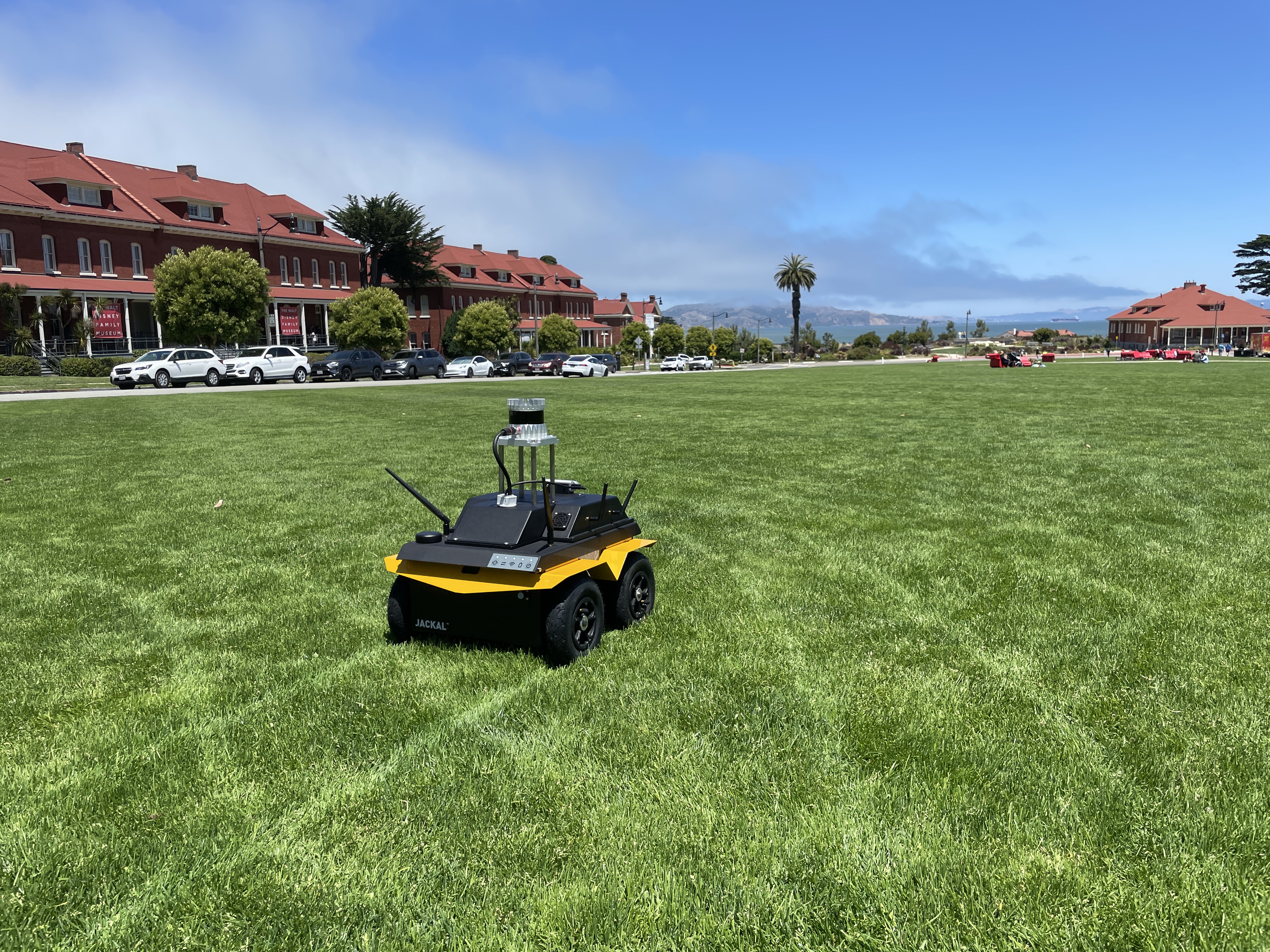
This package contains a series of real-world applicable demos based on ROS 2 Humble. These demonstrations include Outdoor GPS Patrolling, Outdoor 3D Urban Navigation, and 2D Indoor Long-Duration Picking. We use an AMD Ryzen CPU (60W) with advanced NPU and AI Accelerator for these demonstrations, which are well up to the challenge of image and 3D lidar processing with much room left over for user applications and AI.
They are also great entry points for robotics applications to show how to setup a robot system, configure Nav2 for a variety of non-trivial situations, and design a proof of concept autonomy script for research, startups, or prototypers!
⚠️ Need ROS 2, Nav2 help or support? Contact Open Navigation! ⚠️
Demo 1: High-Speed, Outdoor GPS Navigation
The goal of this demonstration is to navigate outdoors in a non-planar environment running Nav2 at full speed - 2m/s. This is performed on the Presidio main parade lawn in San Francisco, CA because it is a beautiful, generally empty, wide open space in which the robots can be let loose at high speeds safely. This demonstration uses GPS to localize the robot while performing a patroling task in a loop and taking some measurements at each point of interest. There is no map what so ever.
Note: Click on the image above to see the GPS Patrol demo in action on YouTube!
For more information, options, and a tutorial on GPS Navigation with Nav2, see the Nav2 GPS Waypoint Navigation tutorial.
Technical Summary
Demo 1 uses robot_localization for GPS handling and sensor fusion. The datum for robot_localization is set to be an arbitrarily selected position on the park to ground the localization system near the origin for convenience and such that this application can be repeated using the same waypoints grounded to a consistent coordinate system, as would be necessary for a deployed application. The experiment was performed over multiple sessions and days.
It also leverages the nav2_waypoint_follower package to follow waypoints in the cartesian frame setup, though can also be done with direct GPS points as well in ROS 2 Iron and newer. It pause a few seconds at each waypoint to capture patrol data using the waypoint follower’s task executor plugins.
A few important notes on this demonstration’s configuration:
- Since we’re navigating in non-flat, outdoor 3D spaces, we use a node to segment the ground out from the pointclouds for use in planning/control rather than directly feeding them in with the 3D terrain variations.
- The controller is configured to run at the robot’s full speed, 2 m/s. This speed should be used by professionals under supervision if there is any chance of collision with other people or objects. These are dangerous speeds and require attention.
- The planner uses the Smac Planner Hybrid-A* so we can set a conservative maximum turning radius while operating at those speeds so the robot doesn’t attempt to flip over due to its own centripetal force. It uses RPP to follow this path closely.
- The global costmap is set to a rolling, static size rather than being set by a map’s size or static full field area. This is likely the best configuration for GPS Navigation when not using a map, just ensure that it is sufficiently large to encompass any two sequential viapoints.
- This demonstration uses a BT that will not replan until its hit its goal or the controller fails to compute trajectories to minimize the impact of ~1-3m localization jumps on robot motion. This prevents ‘drunken’ behavior due to non-corrected GPS data’s noise.
- The positioning tolerances are set comparatively high at 3m due to the noisy non-RTK corrected GPS. Additionally, the perception modules are configured as non-persistent so that the major jumps in localization don’t cause series issues in planning for the world model - we use a 3D lidar, so we have good real-time 360 deg coverage. Both of these could be walked back when using RTK for typical uses of Nav2 with GPS localization.
Dataset
The raw data from the robot during an approximately ~5 minute patrol loop including odometry, TF, commands, sensor data, and so forth can be downloaded in this link.
An example loop of the full length of the parade lawn with noisy GPS data can be seen below for illustration purposes. Navigation can still be leveraged effectively, however please be realistic about the limits on positional accuracies possible. GPS without RTK can obtain about 3-5m accuracy, but will jump:
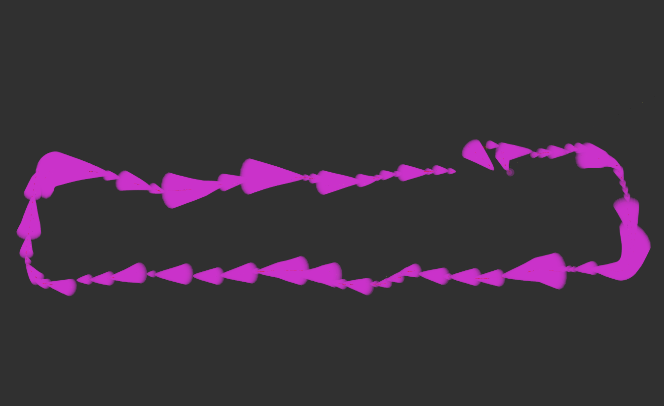
This can be reproduced with the provided rosbag of odometry, GPS data for state estimation.
ros2 bag play initial_gps_loop_rosbag.db3 --clock 20
ros2 launch honeybee_nav2 gps_localization.launch.py use_sim_time:=True
Notes on GPS
For this demonstration, a cheap built-in non-RTK corrected, single antenna GPS is used to localize the robot to show how to work with Nav2 outdoor with noisy GPS localization. For a refined application, an RTK corrected, dual antenna GPS sensor is recommended to improve accuracy of localization, positioning tolerances, and allow for persistence of perception data without major jumps. There are many affordable RTK GPS sensors on the market, for example.
With the GPS, its good to let the robot sit with the filter running for a little while before starting up the demo for the filter to converge to its location solidly before starting. I’ve noticed driving around a little bit to help with that process and converge the orientation from the IMU data.
Demo 2: High-Speed, Urban 3D Navigation
The goal of this demonstration is to show the system in action running Nav2 using 3D SLAM and localization in an urban setting. This is performed on Alameda, an island in the San Francisco bay, because it has a large urban area formerly hosting a Naval Air Station which is perfect for experimentation without much through-traffic (and generally kind, understanding people). This demonstration maps and localizes the robot within a few city blocks on Alameda and routes the robot along the roadways using a navigation graph to go from one building to another representing an urban-navigation use-case.

Note: Click on the image above to see the Urban Navigation demo in action on YouTube!
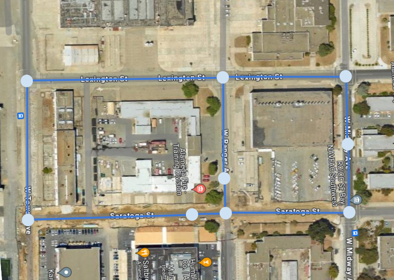
This is the experiment’s location on Alameda & drone footage show the area for scale. The loop is approximately 1 km in length and takes the robot about 10 minutes to navigate around the outside bounding loop. The navigation graph routes through and/or visit a few intersections, a very nice brewery, Alameda’s city hall, and a fire training station. For the purposes of the video demonstration, street nodes are used as routes to get us to final destinations (city hall, brewery, station). The demonstration’s autonomy script by default will randomly select a location to visit including intersections to provide more randomization.
Technical Summary
We use lidarslam_ros2 for 3D SLAM and lidar_localization_ros2 SLAM using the Ouster 3D lidar. The OS-0 has a lower range than its OS-1 and OS-2 counterparts (in exchange for a wide vertical FOV), thus this demonstration is performed in an area where buildings and structures can be effectively seen within the limited ~30 meter effective range.
A few important notes on this demonstration’s configuration:
- Since we’re navigating in non-flat, urban 3D spaces, we use a node to segment the ground out from the pointclouds for use in planning/control rather than directly feeding them in with the 3D terrain variations. Some of the streets have large potholes, tall curbs, and small hills.
- In this demonstration, we use a navigation route graph of the streets and blocks for long-term planning in place of freespace planning on the roadways (i.e. like Google Maps or an AV might route). It computes the most time-optimal route on the roadway graph to get to a destination node. For a deployed application, you may marry this with the Nav2 freespace planner (like shown in the GPS demonstration above) to go the ‘last meters’ off the roads/sidewalks for the final positioning.
- Nav2’s path smoother is used to smooth out the 90 degree turns in the graph to make better use of the roadway intersections and smooth, intuitive motion.
- The controller is configured to run at the robot’s full speed, 2 m/s to operate on public roadways. This speed and operating on public roads should be used by professionals under careful supervision of the robot and environment around you. It is recommended to follow the robot closely and be ready to take over to pause in case through traffic appears. Be courteous and thoughtful in public spaces. We use DWB for this demonstration to round off the use of all 3 major controllers in the demos.
- The positioning tolerances are set to be 50cm due to the good accuracy of the 3D localization (opposed to uncorrected GPS).
- STVL is used now that localization is accurate to mark and raytrace data for managing a proper environmental model (with a temporal element).
An easy workflow to reproduce:
- Teleop robot to create map (or using autonomous navigation). Save map.
- Using Rviz or another tool, find the location of key points of interest and intersections.
- Update the graph to contain these intersections or points of interest based on the map’s coordinate system.
- Launch the demo and localize the robot in the 3D map, making sure that there is good correspondances between the map and sensor data before starting
- Start the demo to go to random locations or modify to send it on a particular route!
Dataset
The raw data from a 3D mapping run around the entire 2 city block area can be downloaded in this link. Unfortunately, due to settings or limitations of the rosbags, some of the 3D lidar data does not appear to have been properly captured in some high-load moments of the experiment due to its length, but there are plenty of good segments.
Notes on 3D Mapping, Planning
For this demonstration, several 3D SLAM and localization solutions were analyzed. Unfortunately, relatively few were robust enough for use and the 3D SLAM selected was the best performing for the robot’s OS-0 and its range sensor limitations. While ‘good enough’ success was found with this method, it is easy to swap in another solution that you prefer.
Planning in Urban spaces can be done 2 primary ways (or mixed for long term & short term planning):
- Using freespace algorithms like the NavFn or Smac Planners which allow for planning in all non-occupied spaces constrained by some behavioral constraints like inflation, keepouts, semantics, or higher cost regions
File truncated at 100 lines see the full file
Package Dependencies
| Deps | Name |
|---|---|
| rclpy | |
| honeybee_watchdogs | |
| honeybee_bringup | |
| honeybee_nav2 | |
| opennav_docking | |
| ament_copyright | |
| ament_flake8 | |
| ament_pep257 |
System Dependencies
| Name |
|---|
| python3-pytest |
Dependant Packages
Launch files
Messages
Services
Plugins
Recent questions tagged honeybee_demos at Robotics Stack Exchange
|
|
honeybee_demos package from opennav_amd_demonstrations repohoneybee_bringup honeybee_demos honeybee_description honeybee_gazebo honeybee_nav2 honeybee_watchdogs |
ROS Distro
|
Package Summary
| Tags | No category tags. |
| Version | 1.0.0 |
| License | Apache 2.0 |
| Build type | AMENT_PYTHON |
| Use | RECOMMENDED |
Repository Summary
| Description | Project containing demonstrations using AMD's Ryzen AI and other technologies with ROS 2 |
| Checkout URI | https://github.com/open-navigation/opennav_amd_demonstrations.git |
| VCS Type | git |
| VCS Version | main |
| Last Updated | 2024-08-26 |
| Dev Status | UNKNOWN |
| Released | UNRELEASED |
| Tags | No category tags. |
| Contributing |
Help Wanted (-)
Good First Issues (-) Pull Requests to Review (-) |
Package Description
Additional Links
Maintainers
- Steve Macenski
Authors
Honeybee Demos
This package contains a series of real-world applicable demos based on ROS 2 Humble. These demonstrations include Outdoor GPS Patrolling, Outdoor 3D Urban Navigation, and 2D Indoor Long-Duration Picking. We use an AMD Ryzen CPU (60W) with advanced NPU and AI Accelerator for these demonstrations, which are well up to the challenge of image and 3D lidar processing with much room left over for user applications and AI.
They are also great entry points for robotics applications to show how to setup a robot system, configure Nav2 for a variety of non-trivial situations, and design a proof of concept autonomy script for research, startups, or prototypers!
⚠️ Need ROS 2, Nav2 help or support? Contact Open Navigation! ⚠️
Demo 1: High-Speed, Outdoor GPS Navigation
The goal of this demonstration is to navigate outdoors in a non-planar environment running Nav2 at full speed - 2m/s. This is performed on the Presidio main parade lawn in San Francisco, CA because it is a beautiful, generally empty, wide open space in which the robots can be let loose at high speeds safely. This demonstration uses GPS to localize the robot while performing a patroling task in a loop and taking some measurements at each point of interest. There is no map what so ever.
Note: Click on the image above to see the GPS Patrol demo in action on YouTube!
For more information, options, and a tutorial on GPS Navigation with Nav2, see the Nav2 GPS Waypoint Navigation tutorial.
Technical Summary
Demo 1 uses robot_localization for GPS handling and sensor fusion. The datum for robot_localization is set to be an arbitrarily selected position on the park to ground the localization system near the origin for convenience and such that this application can be repeated using the same waypoints grounded to a consistent coordinate system, as would be necessary for a deployed application. The experiment was performed over multiple sessions and days.
It also leverages the nav2_waypoint_follower package to follow waypoints in the cartesian frame setup, though can also be done with direct GPS points as well in ROS 2 Iron and newer. It pause a few seconds at each waypoint to capture patrol data using the waypoint follower’s task executor plugins.
A few important notes on this demonstration’s configuration:
- Since we’re navigating in non-flat, outdoor 3D spaces, we use a node to segment the ground out from the pointclouds for use in planning/control rather than directly feeding them in with the 3D terrain variations.
- The controller is configured to run at the robot’s full speed, 2 m/s. This speed should be used by professionals under supervision if there is any chance of collision with other people or objects. These are dangerous speeds and require attention.
- The planner uses the Smac Planner Hybrid-A* so we can set a conservative maximum turning radius while operating at those speeds so the robot doesn’t attempt to flip over due to its own centripetal force. It uses RPP to follow this path closely.
- The global costmap is set to a rolling, static size rather than being set by a map’s size or static full field area. This is likely the best configuration for GPS Navigation when not using a map, just ensure that it is sufficiently large to encompass any two sequential viapoints.
- This demonstration uses a BT that will not replan until its hit its goal or the controller fails to compute trajectories to minimize the impact of ~1-3m localization jumps on robot motion. This prevents ‘drunken’ behavior due to non-corrected GPS data’s noise.
- The positioning tolerances are set comparatively high at 3m due to the noisy non-RTK corrected GPS. Additionally, the perception modules are configured as non-persistent so that the major jumps in localization don’t cause series issues in planning for the world model - we use a 3D lidar, so we have good real-time 360 deg coverage. Both of these could be walked back when using RTK for typical uses of Nav2 with GPS localization.
Dataset
The raw data from the robot during an approximately ~5 minute patrol loop including odometry, TF, commands, sensor data, and so forth can be downloaded in this link.
An example loop of the full length of the parade lawn with noisy GPS data can be seen below for illustration purposes. Navigation can still be leveraged effectively, however please be realistic about the limits on positional accuracies possible. GPS without RTK can obtain about 3-5m accuracy, but will jump:
This can be reproduced with the provided rosbag of odometry, GPS data for state estimation.
ros2 bag play initial_gps_loop_rosbag.db3 --clock 20
ros2 launch honeybee_nav2 gps_localization.launch.py use_sim_time:=True
Notes on GPS
For this demonstration, a cheap built-in non-RTK corrected, single antenna GPS is used to localize the robot to show how to work with Nav2 outdoor with noisy GPS localization. For a refined application, an RTK corrected, dual antenna GPS sensor is recommended to improve accuracy of localization, positioning tolerances, and allow for persistence of perception data without major jumps. There are many affordable RTK GPS sensors on the market, for example.
With the GPS, its good to let the robot sit with the filter running for a little while before starting up the demo for the filter to converge to its location solidly before starting. I’ve noticed driving around a little bit to help with that process and converge the orientation from the IMU data.
Demo 2: High-Speed, Urban 3D Navigation
The goal of this demonstration is to show the system in action running Nav2 using 3D SLAM and localization in an urban setting. This is performed on Alameda, an island in the San Francisco bay, because it has a large urban area formerly hosting a Naval Air Station which is perfect for experimentation without much through-traffic (and generally kind, understanding people). This demonstration maps and localizes the robot within a few city blocks on Alameda and routes the robot along the roadways using a navigation graph to go from one building to another representing an urban-navigation use-case.
Note: Click on the image above to see the Urban Navigation demo in action on YouTube!
This is the experiment’s location on Alameda & drone footage show the area for scale. The loop is approximately 1 km in length and takes the robot about 10 minutes to navigate around the outside bounding loop. The navigation graph routes through and/or visit a few intersections, a very nice brewery, Alameda’s city hall, and a fire training station. For the purposes of the video demonstration, street nodes are used as routes to get us to final destinations (city hall, brewery, station). The demonstration’s autonomy script by default will randomly select a location to visit including intersections to provide more randomization.
Technical Summary
We use lidarslam_ros2 for 3D SLAM and lidar_localization_ros2 SLAM using the Ouster 3D lidar. The OS-0 has a lower range than its OS-1 and OS-2 counterparts (in exchange for a wide vertical FOV), thus this demonstration is performed in an area where buildings and structures can be effectively seen within the limited ~30 meter effective range.
A few important notes on this demonstration’s configuration:
- Since we’re navigating in non-flat, urban 3D spaces, we use a node to segment the ground out from the pointclouds for use in planning/control rather than directly feeding them in with the 3D terrain variations. Some of the streets have large potholes, tall curbs, and small hills.
- In this demonstration, we use a navigation route graph of the streets and blocks for long-term planning in place of freespace planning on the roadways (i.e. like Google Maps or an AV might route). It computes the most time-optimal route on the roadway graph to get to a destination node. For a deployed application, you may marry this with the Nav2 freespace planner (like shown in the GPS demonstration above) to go the ‘last meters’ off the roads/sidewalks for the final positioning.
- Nav2’s path smoother is used to smooth out the 90 degree turns in the graph to make better use of the roadway intersections and smooth, intuitive motion.
- The controller is configured to run at the robot’s full speed, 2 m/s to operate on public roadways. This speed and operating on public roads should be used by professionals under careful supervision of the robot and environment around you. It is recommended to follow the robot closely and be ready to take over to pause in case through traffic appears. Be courteous and thoughtful in public spaces. We use DWB for this demonstration to round off the use of all 3 major controllers in the demos.
- The positioning tolerances are set to be 50cm due to the good accuracy of the 3D localization (opposed to uncorrected GPS).
- STVL is used now that localization is accurate to mark and raytrace data for managing a proper environmental model (with a temporal element).
An easy workflow to reproduce:
- Teleop robot to create map (or using autonomous navigation). Save map.
- Using Rviz or another tool, find the location of key points of interest and intersections.
- Update the graph to contain these intersections or points of interest based on the map’s coordinate system.
- Launch the demo and localize the robot in the 3D map, making sure that there is good correspondances between the map and sensor data before starting
- Start the demo to go to random locations or modify to send it on a particular route!
Dataset
The raw data from a 3D mapping run around the entire 2 city block area can be downloaded in this link. Unfortunately, due to settings or limitations of the rosbags, some of the 3D lidar data does not appear to have been properly captured in some high-load moments of the experiment due to its length, but there are plenty of good segments.
Notes on 3D Mapping, Planning
For this demonstration, several 3D SLAM and localization solutions were analyzed. Unfortunately, relatively few were robust enough for use and the 3D SLAM selected was the best performing for the robot’s OS-0 and its range sensor limitations. While ‘good enough’ success was found with this method, it is easy to swap in another solution that you prefer.
Planning in Urban spaces can be done 2 primary ways (or mixed for long term & short term planning):
- Using freespace algorithms like the NavFn or Smac Planners which allow for planning in all non-occupied spaces constrained by some behavioral constraints like inflation, keepouts, semantics, or higher cost regions
File truncated at 100 lines see the full file
Package Dependencies
| Deps | Name |
|---|---|
| rclpy | |
| honeybee_watchdogs | |
| honeybee_bringup | |
| honeybee_nav2 | |
| opennav_docking | |
| ament_copyright | |
| ament_flake8 | |
| ament_pep257 |
System Dependencies
| Name |
|---|
| python3-pytest |